Flowing between Python and SQL
Dataframe SQL lets you run SQL queries on any dataframes in a Hex project, including the results of previous SQL queries. Sometimes you need to dip into Python for a moment, but don't want to abandon SQL entirely. With Dataframe SQL in Hex you can chain SQL and Python together, which allows for a lot of flexibility.
This tutorial explains how to use Dataframe SQL to do a quick intermediate python step between two SQL queries. We'll run a SQL query, drop into Python to do some geocoding on that same dataset, and then return back to SQL to efficiently get a subset of the data ready for visualization.
This tutorial is available as a published Hex App here.
Step 1: SQL query
We'll query a demo e-commerce dataset and return a whole bunch of information about orders, including the city they used for a shipping address.
Check out the Notebook view for the real SQL cell - this is just a code snippet in markdown.
SELECT
order_id,
order_date,
customer_name,
category,
sales,
profit,
COALESCE(city,' ') || ', ' || COALESCE(state, ' ') || ', ' || COALESCE(postal_code, ' ') || ', ' ||COALESCE(country,' ') AS address
FROM public.superstore_dataset
LIMIT 100
Step 2: Geocoding in Python
Looks good! But the address data isn't really enough to do any kind of analytics on. We'd like to know how far each user's shipping address is from our warehouse in Santa Cruz, California and you can't just do DISTANCE(Santa Cruz CA, Luanda Angola), as cool as that would be.We need to enrich this data somehow.
This is one of those things that Python's ecosystem is perfectly set up to help with. Let's drop out to Python and use the geopy library. We instantiate a new geopy geocoder and give it a user agent, then apply the geocoder to the entire dataframe. The query is just 100 rows for demo purposes, so as not to overload the free geocoding service (thank you!)
# Instantiate a geocoder and give it a user agent.
locator = Nominatim(user_agent="hex-geocoder")

# Apply the geocoder to the entire dataframe (just 100 rows for demo purposes, thank you free Geocoding service!)
orderdata['location'] = orderdata['address'].apply(locator.geocode)
The geocoding returns a point object, which needs to be split up into lat/long, so we do a tiny bit more transformation in python and then return the latitude and longitude as individual columns.
orderdata['point'] = orderdata['location'].apply(lambda loc: tuple(loc.point) if loc else None)

orderdata[['latitude', 'longitude', 'altitude']] = pd.DataFrame(orderdata['point'].tolist(), index=orderdata.index)
Then we're ready to calculate the distance! We'll use the great_circle distance, and apply that function to the entire dataframe. The np.isfinite() call is just checking for null values, since there's a couple rows we couldn't geocode.
hq_loc = (36.97307082021759, -122.01929189549323)

orderdata['distance_from_hq'] = orderdata.apply(lambda row: great_circle((row['latitude'],row['longitude']), hq_loc).miles if np.isfinite(row['latitude']) else None , axis=1)
Step 3: Back to SQL
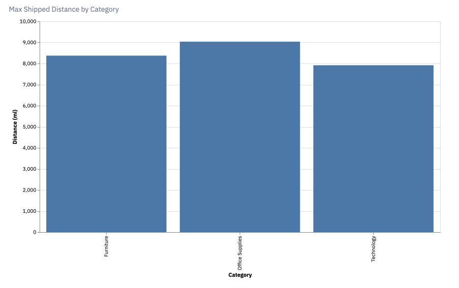
Let's jump back into SQL where it's a bit easier to grab subsections of the data. We'll write one more simple query and then chart the result:
SELECT
order_id,
category,
profit,
MAX(distance_from_hq) AS distance
FROM orderdata
GROUP BY 1,2,3
ORDER BY 2 DESC
To create a chart of the results, add a Chart cell. Leave it as the default bar graph format then update the data source to distancedata. Set category as the X-axis and distance as the Y-axis and the bar chart should populate. If you’re making this chart for your own project, you’ll be able to customize the chart’s axes, colors, and other configurations (see the documentation here).
