SQL cells

Query your warehouse, CSVs, or Pandas dataframes with SQL. Reference the results of your query in downstream cells to create sophisticated, and dynamic, chains of logic.

info

• Users need Can Edit permissions to create and edit SQL cells.

SQL cells run queries and return the results as a variable that can be used in downstream cells.

These results can be used in Chart, Pivot, SQL, and other cells. This allows you to create chains of logic, linking together queries, visualizations, dynamic inputs, and more.

SQL cells can also be parameterized with Jinja, unlocking workflows like filtering data based on the value of an input cell.

Choose a data source

First, create a SQL cell and select a data source in the top right corner. SQL cells can query two types of data sources: warehouse connections (to query tables and views in your data warehouse) and dataframes (to query in-memory dataframes and CSVs using DuckDB).

Warehouse connections

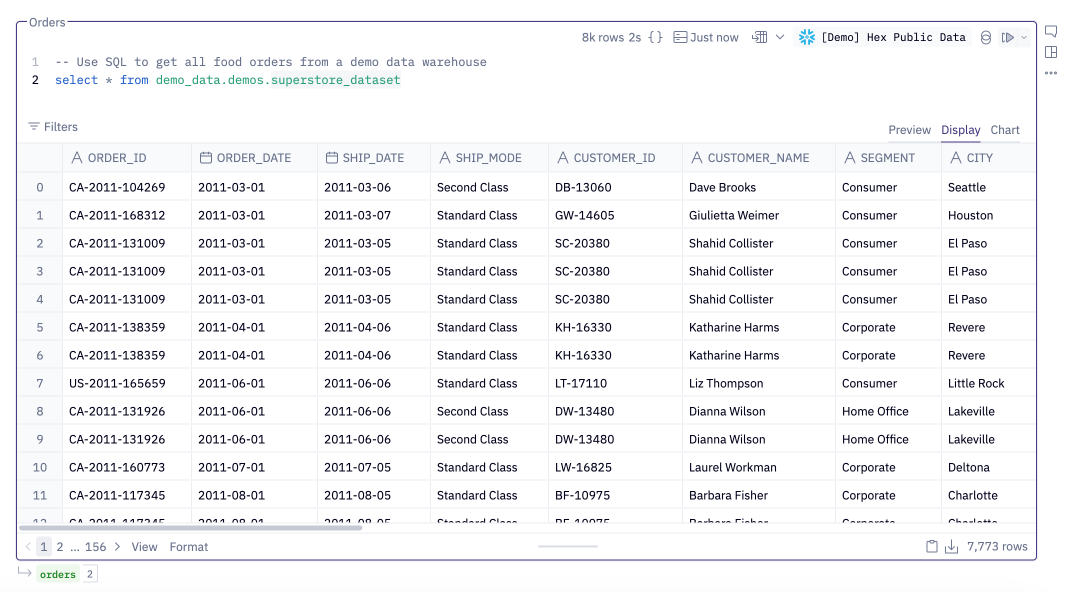
To query tables and views in your data warehouse, choose a warehouse connection as the data source.

An admin in your workspace has likely set up a workspace data connection that lets you connect to your organization's data warehouse.

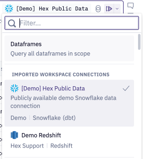
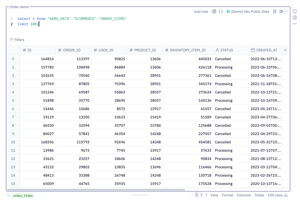
You can then write SQL directly in the cell, using the SQL dialect of the selected connection:

Additionally, if you have credentials to a data warehouse, you can create a project data connection that is scoped only to the current project.

Note: Users on the Enterprise plan may not be able to create project data connections if the option has been disabled by an admin.

Dataframes

Dataframe SQL allows you to write SQL that references any dataframes or uploaded CSVs in your project.

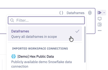
Dataframes in your project may have been created with Python cells or returned by a SQL cell within the same project.

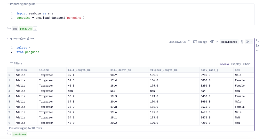
When using Dataframe SQL, you'll need to use the DuckDB dialect of SQL. Reference any dataframe in the FROM or JOIN clauses, using the dataframe name where you would normally use a table name.

Dataframe SQL can also query CSV files in your project. First, upload a .csv file, then write SQL that references the file name, for example: SELECT * FROM "file_name.csv".

Run queries

Once you've selected a data source and written your SQL, use ⌘ + Enter (or Ctrl + Enter on a PC) to run the query. You can also click the Run button in the top right corner of the cell.

Return results as a variable

SQL cells return their results as a variable that can be used in downstream cells.

This variable can be renamed to improve project readability. To rename a result, click the current name and type a new one. Renaming a result automatically updates all downstream references.

Warehouse SQL cells

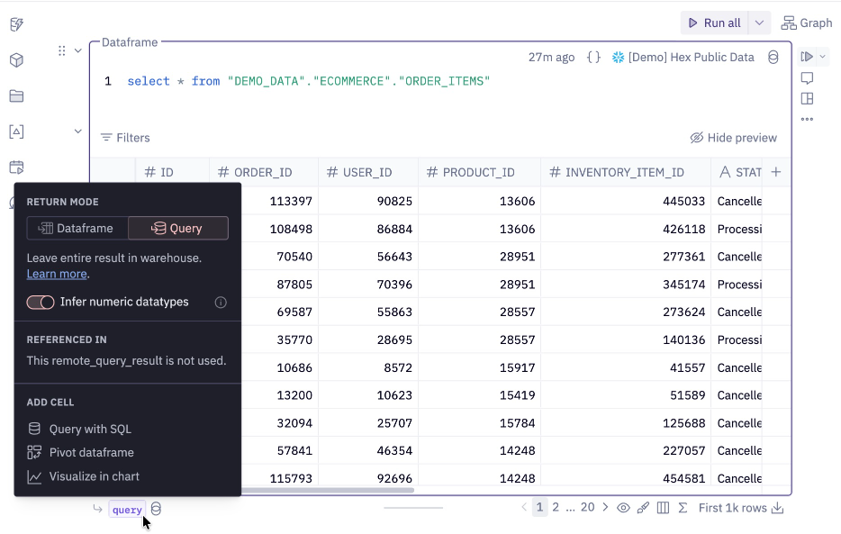
Warehouse SQL cells can return results as a dataframe or as a query.

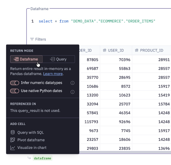
When dataframe is selected (the default), the output will be shown as a green pill. In this mode, SQL cells stream all results of the query from your warehouse to Hex, which can then be used in downstream cells as a Pandas dataframe.

info

If your dataset is large (>100k rows), streaming all records may take significant time. Consider using query mode in this case.

You can alternatively return a result as a Query object, and the output will be shown as a purple pill. In this mode, SQL cells only fetch a preview of data (the first 1k rows). The output can still be used downstream, if those cells can be compiled to warehouse SQL. This includes referencing the result in another warehouse SQL cell, or in a Chart cell that applies an aggregation that can be expressed as warehouse SQL.

Query mode is useful if you're working with large amounts of data — learn more below.

The output of a warehouse SQL cell always includes the query text itself, which can be referenced downstream in other SQL cells. This is referred to as chained SQL, more information below.

Dataframe SQL cells

Dataframe SQL cells always return results as a Pandas dataframe (shown as a green pill). These results can be referenced in any cell that works with dataframes, such as other dataframe SQL cells or Python cells.

Use SQL results in other cells

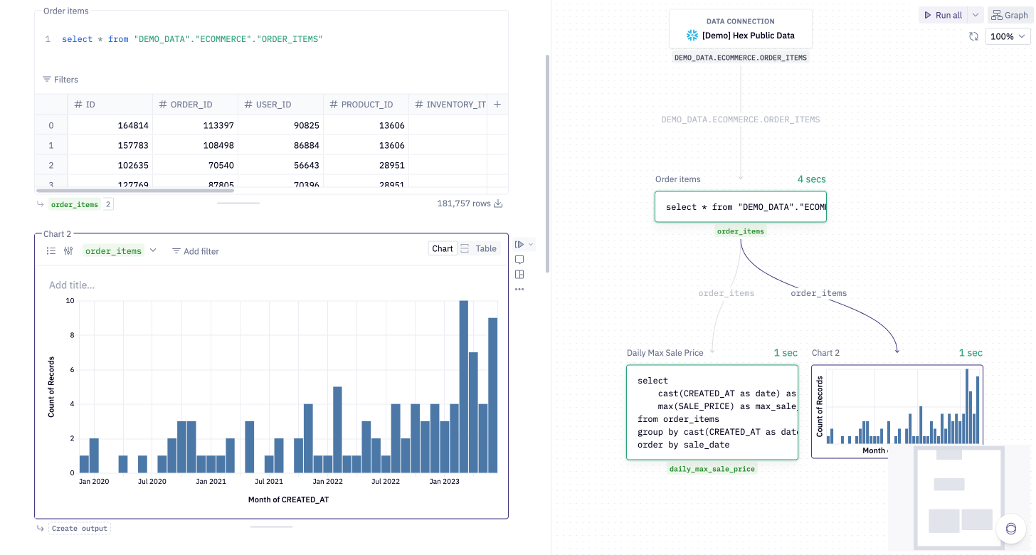
Since SQL cells return results as a variable, these variables can be referenced in other cells to create a DAG (directed acyclic graph) of cells.

In warehouse SQL cells

You can reference the result of a previous warehouse SQL cell in other warehouse SQL cells by using the upstream variable name where you would typically use a table name. This is often the most natural way to link queries together — it allows you to stay in one dialect of SQL and seamlessly flow between cells.

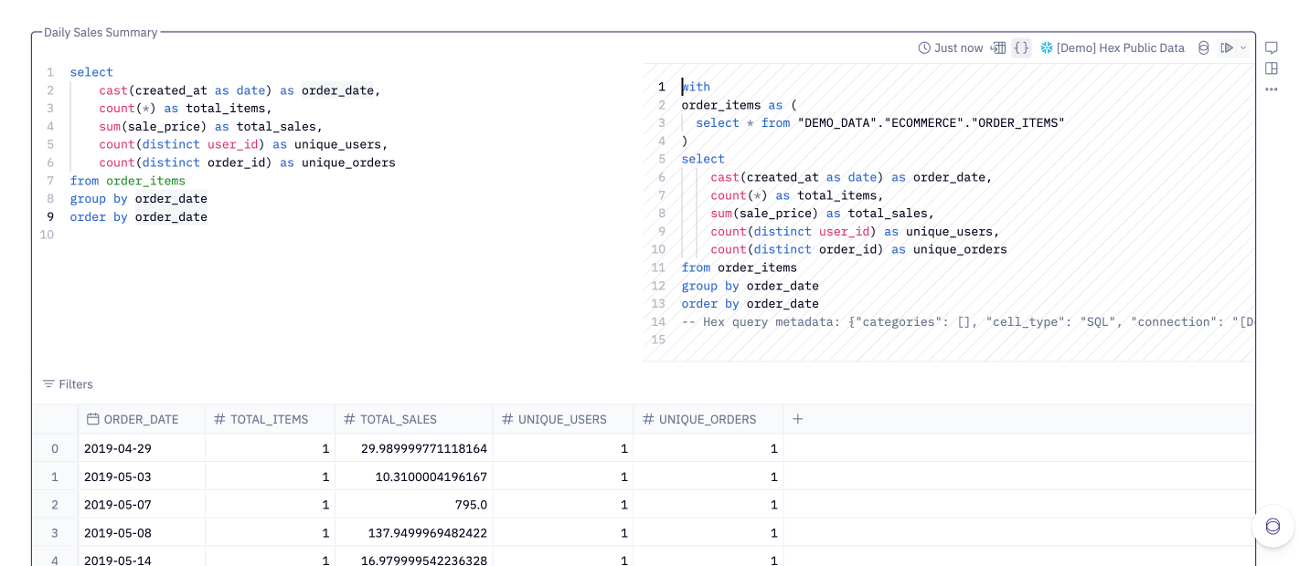
Behind the scenes, Hex inserts your upstream SQL as a CTE (common table expression) at the start of the query. You can see the generated SQL via the View compiled SQL option in the top-right corner.

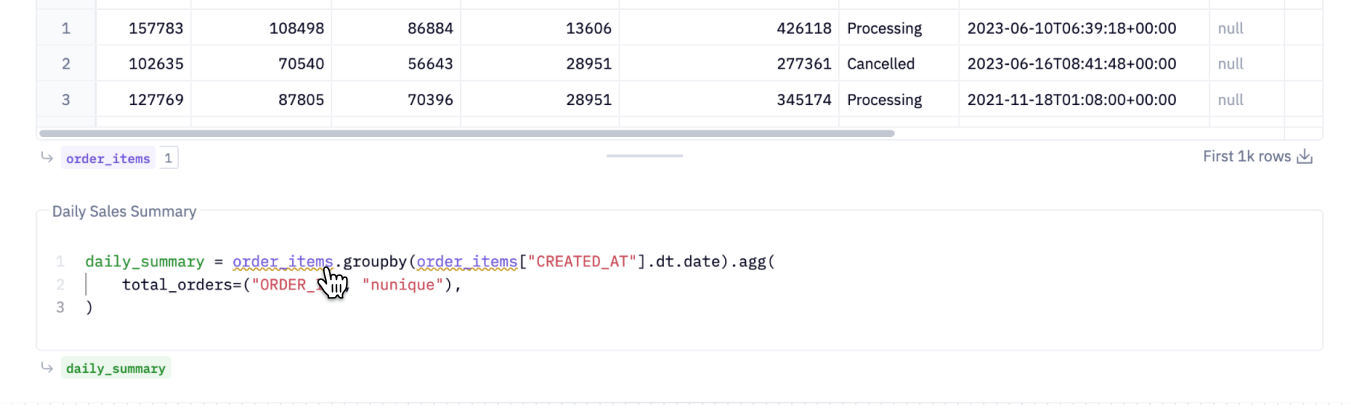
In dataframe SQL cells

Dataframe SQL cells can reference any dataframes in your project by using the dataframe name where you would typically use a table name.

info

Since warehouse SQL cells (by default) return both a dataframe and a query, you can often choose to query them in either dataframe SQL or warehouse SQL. Learn when to use each approach.

In Python cells

You can reference the result of a SQL cell in a Python cell using Python code that works with Pandas dataframes.

tip

If you're using Python to perform an operation that could be written in SQL, consider writing it in SQL instead. Staying in SQL allows Hex to perform additional optimizations to improve performance.

In Markdown & Text cells

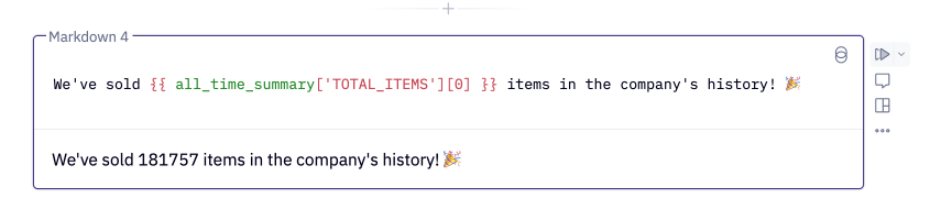
You can use the result of a SQL cell in a Markdown or Text cell, for example, to reference a query result in a summary.

To do this, use Jinja combined with Pandas syntax to access an individual value.

Learn more about dynamic text.

Parameterize SQL cells

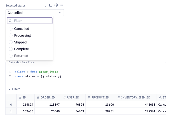
Variables from other parts of your project can be inserted into SQL queries using Jinja templating.

This lets you parameterize queries based on user input, such as applying a where clause dynamically, allowing you to build sophisticated user-facing data applications.

Learn more about SQL parameterization.

Query mode

Warehouse SQL cells can return results as a Dataframe or a Query. When Query is selected, the result pill will turn to purple. In this mode, only a preview of data is fetched (the first 1k rows), which significantly reduces time spent streaming large datasets.

Despite only fetching a preview, query results can still be used in downstream cells that work with warehouse SQL, including other warehouse SQL cells (via chained SQL) and no-code cells like Chart, Pivot, and Single Value cells.

When a query result is used downstream, Hex inserts your SQL as a CTE (common table expression), ensuring the full result set is queried — not just the 1k row preview.

Query result cell compatibility

Query results can be used in all cells in Hex that work with dataframes.

Cell type	Compatible with dataframe	Compatible with query result
Warehouse SQL cell	🟡	✅¹
Dataframe SQL cell	✅	🟡
Python cell	✅	🟡
Chart cell	✅	✅
Pivot cells	✅	✅
Input cell	✅	✅
Single value cell	✅	✅
Table display cell	✅	✅
Filter cell	✅	✅
Markdown & text cells	✅	🟡
Writeback cell	✅	🟡²

Cells that have a ✅ for both dataframe and query result use SQL to perform the transformations required by the cell (for example, aggregations in a Chart cell):

• When the cell uses a dataframe as its input, the required SQL is written in DuckDB and executed on the dataframe in the kernel.
• When the cell uses a query result as its input, the required SQL is written in your warehouse dialect and sent to your warehouse to be executed.

Warehouse SQL cells can reference dataframes that were produced by another warehouse query, but not dataframes that were created with Python cells, as these cannot be expressed as warehouse queries.

Cells that have a ✅ for dataframes but a 🟡 for query results require the full dataframe (for example, using the result in a Python cell). To improve interoperability, you can still reference query results in these cells, but Hex will first fetch the full result set as a dataframe before running the cell. This can lead to significantly more execution time and effectively undoes the optimization benefits of query mode.

In this scenario, references to the query result will show up with a yellow line under the query reference, with an explanation in a tooltip on hover.

If you're using a query result in one of these cells, consider changing the upstream SQL cell to dataframe mode — this makes it clearer when slow execution is caused by streaming results.

¹The warehouse SQL cell must use the same connection as the connection used in the upstream SQL cell.

²Consider using a create table as statement in this scenario.

When should I use query mode?

Use query mode when you're querying large amounts of data (≳100k rows), for the following reasons:

• Reduces time spent streaming data: In dataframe mode, Hex streams all records from your warehouse, which can take significant time (upwards of a minute) for large datasets. In query mode, Hex only fetches a 1k row preview.
• Reduces memory pressure: Each Hex project has a fixed amount of memory, and returning large amounts of data may exceed that limit, resulting in an "Out of memory" error.
• Leverages warehouse performance: When query results are used in no-code cells like Chart or Pivot, Hex pushes the transformations to your warehouse. A well-resourced analytical warehouse is often faster at performing queries on large datasets than running equivalent queries in DuckDB on the kernel.

When should I use dataframe mode?

Use dataframe mode if:

• You need to reference the result in a Python cell — for example, to perform predictive analysis or data manipulation that cannot be expressed in SQL.
• Your datasets are small — for smaller datasets (typically under 100k rows), it's faster, and cheaper, to run queries in DuckDB than to make the round trip to your warehouse.

Fetching row counts

In query mode, only the first 1k rows are returned, so Hex doesn't know the total row count. You can fetch the row count manually, which executes an additional select count(*) query on your result set.

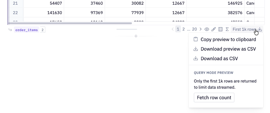
This query can be slow for large result sets, which is why the row count is not fetched by default.

Hiding query previews

You can hide the preview of results in query mode cells.

The query will still be available to use downstream, but Hex won't fetch the 1k row preview on execution. This is useful when fetching the preview takes significant time.

Run behavior of SQL cells

SQL cells in Hex run differently compared to other SQL-based tools.

Reactive execution

When you rerun a SQL cell, all downstream cells that reference its results will automatically re-execute. This is Hex's reactive execution model, which enables fast iteration and immediate feedback loops. Project state stays up to date, even across many SQL, Python, or other cells.

Similarly, if a SQL cell is parameterized with Jinja, changes to the upstream values will cause the SQL cell to rerun automatically.

If needed, you can disable this "Auto" mode and use "Cell only" run mode to prevent reactive execution.

Parallel execution

Since cells in Hex form a DAG (directed acyclic graph), Hex can often run cells in parallel. When multiple warehouse SQL cells can be executed in parallel, Hex sends all parallelizable queries to the warehouse at once and lets your warehouse's query engine process them according to its queueing mechanism.

SQL query caching

Hex caches the results of SQL queries to reduce load on your data warehouse and improve execution time. If the query you're running has been executed recently, Hex serves the cached results rather than going back to the warehouse. Learn more about SQL query caching.

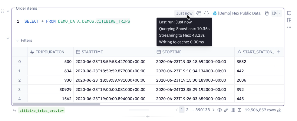
Execution time

When you run a SQL cell in Hex, execution time consists of two main components:

1. Executing your query (including any queueing time in your data warehouse)
2. Streaming results back to Hex

You can see query and streaming time broken down in this tooltip:

More detailed stats are available in Run stats.

Queries in Hex may sometimes be slower than querying directly from your data warehouse's query UI because:

1. Hex needs to establish a connection to your data warehouse, adding a small amount of overhead.
2. If your query returns a large amount of data, streaming those results takes time. In this case, consider query mode.

If the query execution portion is taking longer than expected, ask a database admin to check if your warehouse is experiencing resource contention or if it needs to be scaled for larger workloads.

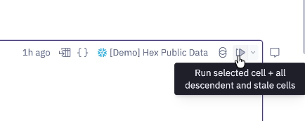
Running selected SQL

For long and complex queries, you can execute only a portion of your SQL by highlighting the text to execute, then using keyboard shortcuts (⌘ + Enter or Ctrl + Enter on a PC) or the cell's run button.

Note that when running selected SQL, downstream cells that reference the SQL cell's result will not run automatically.

Stopping SQL queries

To stop a query, click the loading animation in the upper right of the running cell. This sends a request to the database to cancel the query.

Clicking Stop/Interrupt from the dropdown of a project's run options will also stop any currently-running queries.

If the cell is still queued (tooltip reads "This cell has been queued for execution"), the query hasn't been sent to the database yet. Stopping the project while the cell is still queued will prevent the query from being sent.

info

Requests to stop a SQL query are not always honored by the database immediately. Common causes include the query having already completed by the time the cancel request reaches the database, exhausted warehouse compute resources, or an overloaded task scheduler.

The only way to guarantee that a query won't run against your database is to cancel it while still queued, before it has been sent.

Multi-statement queries & session parameters

Each warehouse SQL cell creates a different database session — this allows Hex to run warehouse queries in parallel, but also means that if you need two SQL statements to run within the same session, they must be written in the same cell.

To do this, write multiple statements in a single SQL cell, separating statements with a semicolon (;).

warning

Note that Athena, Databricks, ClickHouse, & Trino do not support multi-statement queries.

Below is a PostgreSQL example that:

1. Drops a table if it already exists
2. Creates a new table, defining the column names and types.
3. Inserts a row of data into the table
4. Returns the contents of the table.

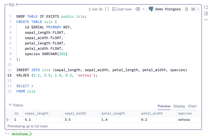
All databases, except for SQL Server, will return the results of the last statement as the output. SQL Server returns the results of the first statement.

FAQs & common workflows

When should I use warehouse SQL vs dataframe SQL?

This decision is often determined by where your data lives:

Query references	Allowed query type
A table or view in a data warehouse	Warehouse SQL
An object that is only available as a dataframe¹	Dataframe SQL
The result of an upstream warehouse SQL cell	Warehouse SQL, or dataframe SQL²
Two datasets from different data sources	Dataframe SQL

¹Examples include:

• A CSV that has been uploaded to a project
• A dataframe that has been mutated with Python (e.g., via Pandas)

²Dataframe SQL should not be used if the upstream SQL cell is in query mode.

When you have the choice between warehouse SQL or dataframe SQL, the right approach depends on your data size and workflow:

Use dataframe SQL when:

• Working with smaller datasets (typically ≲100k rows) — Hex doesn't need to send the query to a warehouse and wait for results, making it faster.
• Note that dataframe SQL requires using the DuckDB dialect of SQL, which may introduce mental overhead or confusion for other users.

Use warehouse SQL when:

• Working with larger datasets, especially when using data warehouses optimized for analytical workloads. The exact threshold where this changes is highly dependent on your warehouse — we typically see that queries that process ≲100k rows are faster in dataframe SQL.
• You want to stay in your warehouse's SQL dialect for consistency.

Querying CSVs

To query a CSV file, first upload it to the files sidebar. Then write dataframe SQL that references the file directly, for example: SELECT * FROM "file_name.csv".

Joining results from two sources

To join data from different data sources, run two warehouse SQL queries and return the results as dataframes. Then use a dataframe SQL cell to join the two dataframes together.

SQL cell reference

Query datatypes

When query results are returned as a Pandas dataframe, some database-specific column types are transformed into Pandas-supported datatypes. Hex keeps these conversions as consistent as possible across database types.

The following mappings are applied:

database column type	pandas column type
int	int
int (with null values)	float
float	float
decimal	float¹
string	object
date	date¹
timestamp	timestamp

¹This behavior can be disabled — see the below sections for more information.

Notable differences between database column types and Pandas data types:

• Any int type column that contains nulls is converted to a float type in the output dataframe, due to how Pandas handles integer columns.
• Decimal-type columns are returned with varying decimal places depending on the database (PostgreSQL: 18, BigQuery: 9, Snowflake: 1).
• Datetimes are converted to Pandas integers at nanosecond precision. The number of nanoseconds required to represent far future dates exceeds the maximum allowable for an integer type. If Hex detects such a large datetime, all datetime columns in the dataframe are converted to an object type to avoid conversion errors.

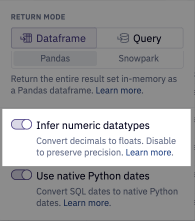
Infer numeric datatypes

When enabled (the default), any column with a decimal type is cast to a float, since Pandas does not support decimal datatypes. This generally makes numbers easier to work with downstream and easier to format in Table display cells.

However, casting a high-precision decimal to a float can result in loss of precision. If precision is critical, you can disable the Infer numeric datatypes option in the SQL cell configuration. When disabled, decimals are represented as an object type instead.

Use native Python dates

When enabled (the default), date columns in a SQL result will be represented as a Date type, with no time, or timezone component, e.g. 2025-09-12. This allows downstream cells, such as Pivot and Chart cells, to handle these values in the expected way. This differs from the standard Pandas dataframe behavior, which represents date columns as Timestamps — there may be a small performance tradeoff when this conversion occurs.

When disabled, date columns are represented as a Timestamp type with both a time and timezone component (midnight UTC), e.g., 2025-09-12 00:00:00+00:00. This aligns with standard Pandas dataframe behavior. Since these columns are timestamps, downstream Pivot and Chart cells will perform timezone conversion based on the hex_timezone value. This often results in data appearing on the "wrong" day, since the timezone conversion may shift the timestamp to a different calendar day (for example, midnight UTC on a Tuesday is still Monday in North and South America).

caution

Disabling this setting can result in unexpected results in downstream Chart and Pivot cells. Only disable this setting when absolutely necessary.

Query metadata

When executing SQL cells, Hex injects a comment into queries that includes metadata about the source: the issuing user's email, a link to the project and cell where the query originated, and the relevant trace ID. This allows database administrators to track and audit queries originating from Hex. To view query metadata, click the curly brace { } icon in the menu at the top of the cell.

Troubleshooting

Troubleshooting chained SQL

Occasionally, Hex may not compile CTE references correctly. To check if this is happening, view the compiled SQL via the View compiled SQL icon.

This is often caused by a CTE sharing a name with a reserved SQL keyword, which prevents the SQL parser from properly replacing the CTE name with the query.

To resolve this, rename any CTEs that use reserved keywords.

Sort order of union queries

When returning a result in query mode, Hex fetches a preview of the first 1001 rows. To achieve this, Hex generally applies a limit 1001 to your query inline, like so:

User query	Hex preview query
select * from stripe_subscriptions order by stripe_customer_id	select * from stripe_subscriptions order by stripe_customer_id limit 1001

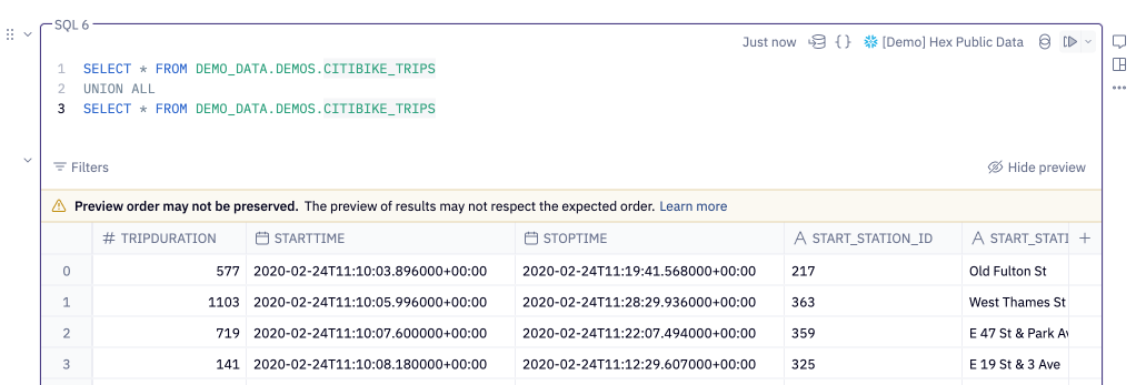
If your SQL cell contains a union statement, Hex instead writes the preview query using a CTE to ensure the correct number of records are fetched.

User query	Hex preview query
select * from retail_customers union all select * from trade_customers	with query as ( select * from retail_customers union all select * from trade_customers ) select * from query limit 1001

When the limit 1001 is applied via a CTE rather than inline, the preview may not respect the ordering defined in the user query — this is a limitation of data warehouses (for example, see Snowflake's documentation on this issue).

In this scenario, we’ll render a warning to let you know that your results may not be ordered correctly.