Develop your notebook
Mix and match SQL, Python, and no-code cells to explore and analyze your data.
- Available on all pricing plans
- Relevant for Admins and Editors with Can Edit or higher project permissions
Hex's Notebook view is built on the familiar notebook format. If you've had experience with Jupyter or similar notebooks, you'll find yourself right at home. Just like in other notebooks, the Notebook view's main interface is composed of cells. However, Hex takes it a step further by offering a range of interactive cell types and expanding on the notebook format in several significant ways. In the following section, we'll delve into how Hex's Notebook view facilitates robust and intuitive data exploration workflows.
Choosing Data
Every great project begins with querying data. You can bring data into your project through a warehouse connection, imported CSV file, or API call. Learn more about connecting your data here.
Data connections
Select the Data sources tab of the left sidebar to see all of the available data connections and their descriptions. Browse the schema of a connected data source by clicking to open it and expanding the section to view the included tables.
To explore the fields in a table, click on the table name and view the metadata as it appears underneath.
If you use dbt Cloud, Hex can use metadata from your dbt project to enrich the Data browser with additional information. Read more about integrating with dbt here.
Select the Query button next to a table to automatically generate a SQL cell and basic query. Edit this query to make it your own!
You can also add a SQL cell by clicking on the green Add Cell button, selecting a data source from the dropdown in the upper left corner of the cell, and writing your query from scratch.
Connecting to and querying a new data source is a quick process from the Data sources tab on the sidebar. Read more about adding new data sources here (link).
Uploaded files
If your data lives in a CSV file, you can upload it from the Files tab of the left sidebar.
Click the three dots next to the filename and select Query in a new SQL cell to automatically generate a basic query.
You can also add a SQL cell using the green Add Cell button and write a query from scratch. Note that you will need to wrap your filename in double quotes (””) for it to query successfully.
Starting with Python
Although many projects start with querying data in SQL and then working with the resulting dataframe in Python, it is possible to skip straight to Python. Add a new Python cell by clicking on the green Add Cell button and write a script to open and read the contents of your CSV file.
import pandas as pd

my_df = pd.read_csv("my_csv_file.csv")

my_df.head()
with open("my_csv_file.csv", "r") as file:
    contents = file.read()
Everything in Hex is a cell
Cells are the building blocks of any Hex project, allowing your project to take shape as you add them.
Cell Types
Hex provides a variety of cell types that let you explore, transform, and share insights about your data:
- Code Cells: Support writing SQL.
- Markdown and Text Cells: Support markdown or text.
- Chart Cells: Support out-of-the-box data visualizations, maps, and interactive tables.
- Transform Cells: Support UI-driven reshaping and filtering of data.
- Input Parameter Cells: Support selecting or setting values interactively.
- Data Cells: Support writing back to a connected database table or bringing in dbt metrics.
Build your logic by adding cells
Adding and updating cells
Add new cells from the Add Cell Bar, or keyboard shortcut command-A to add a new cell above your current position, and command-B to add a new cell below your current position.
In the Outline sidebar in the App builder, you can see all of the cells you added to your project in the Notebook View. Select a cell in the outline and drag it into your App builder to add the cell to your app.
You can also add a new markdown or text cell in the App builder by clicking on the white plus sign at the center bottom of your screen.
You can rearrange cells in your Notebook View by hovering your pointer over the upper left corner of a cell, selecting the cell handle when it appears, and dragging the cell up or down.
To remove a cell, click on the three dots at the upper right corner of the cell and select Delete cell from the menu.
Cell outputs: dataframes and variables
Most Hex cells return variables and/or dataframes that can be referenced in other cells. You can see the variables or dataframes returned by a cell directly beneath the cell. Hover over the variable or dataframe name underneath the cell to see where it’s referenced, and double click to rename it.
Dataframes
Dataframes result from running a new query against your connected data source or executing a query or function that acts on an existing dataframe in your Hex project. Keep track of all the dataframes in your project by viewing them on the Data sources tab of the left sidebar.
For example, when you query data in a SQL cell, the results are stored as a dataframe. This dataframe can then be queried in subsequent SQL cells, referenced in pandas in a Python cell, or be pulled into a Display or Transformation cell. We refer to this as chaining SQL, which you can read more about here.
Variables
Variables result from defining an input in an Input cell, or executing a function in a Code cell.
Once defined, variables can be referenced in other Code, Input Parameter, and Text cells, and in filter fields in Chart and Transform cells. Variables can also be used in SQL cells in combination with Jinja to dynamically run queries or update text.
For example, if you add a Python cell with the function…
def add_five(a_number):
	return 5 + a_number

my_variable = add_five(3)

print(my_variable)
--
8
… the cell will return the output my_variable containing the value 8.
Similarly, if you added a Number Input cell, the cell would return a variable containing the number entered.
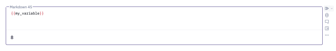
You can then reference my_variable in a Text or Markdown cell by wrapping it in curly braces.
…or in another Code cell.
select *
from my_table
where my_numerical_column > my_variable
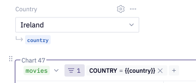
Likewise, you can reference string variables in a filter on a Chart or Transform cell by wrapping it in curly braces. The following example creates the variable country from a dropdown Input parameter and filters a chart based on the value selected.
Chaining Cells
You can chain your logic together across multiple cells by referencing the output of an upstream cell in one further downstream. The best way to explore this is through an example.
Let’s say we have have a SQL query containing two CTEs— CTE A and CTE B— that we then join together. We split each individual CTE into its own SQL cell and add a third SQL cell that performs the join.
As the first SQL cell containing CTE A runs, it returns its result in a dataframe we name df_1.
WITH
    df_1 (cte_col_1, cte_col_2) AS (
        SELECT col_1, col_2
            FROM ...
    )
SELECT ... FROM my_cte;
The second SQL cell containing CTE B runs and returns its result in a dataframe we name df_2.
WITH
    df_2 (cte_col_1, cte_col_2) AS (
        SELECT col_1, col_2
            FROM ...
    )
SELECT ... FROM my_cte;
The third and final SQL cell then runs and references both df_1 and df_2 in its join.
SELECT *
FROM df_1
INNER JOIN df_2 on df_1.col_1 = df2.col_1
We refer to queries that are run against a connected database or warehouse as ‘data connection SQL,’ and queries that run against a local dataframe or CSV as ‘dataframe SQL.’ Read more about the differences between these types of SQL and when to use them in our SQL cells documentation here.
How Cells Run in Hex
Hex maps the relationships between your cells into a graph that helps power its reactive execution model. These linkages are automatically inferred from variable or dataframe references, without any need for user definition. Learn more about our reactive execution compute model here.
We visualize these cell relationships into a Graph view that can be found in your project by clicking on the Graph button. Read more about the Graph view here.
Run modes
The Run mode menu at the top lets you define how the cell executes in notebook view. Projects always run using Auto mode in the app run mode. Read more about run modes here.